Linear regression, famously used by Gauss in 1809 to predict the location of Ceres, is the ur-model of supervised learning.

Suppose $A \in \mathbb{R}^{m \times n}$ with $m \neq n$ and $y \in \mathbb{R}^m$ is a given vector. Find $x \in \mathbb{R}^n$ such that $y = Ax$. $$ $$ However if no $x$ satisfies the equation or more than one $x$ does -- that is the solution is not unique -- the problem is said not to be well posed.

The standard approach in the (overdetermined) case where $m > n$ is linear least squares linear regression. $$ $$ In this situation the linear system $Ax = y$ is not solvable for most values of $y$. $$ $$ The linear least squares problem poses an approximate solution in the following constrained optimization problem:

$$ \min_{b \in \mathcal{Im}(A)} \|y - b\|^2 $$

The SVD gives us a nice way of studying linear systems $Ax = y$ where the matrix is not invertible. $$ $$ In this case $A$ has a generalized inverse called the Moore-Penrose psuedoinverse (denoted $A^+$). $$ $$ The Moore-Penrose psuedoinverse is defined for any real-valued matrix $A$, and corresponds to the normal inverse $A^{-1}$ when $A$ is invertible.

We write $\oplus$ for the direct sum of inner product spaces, $\perp$ for the orthogonal complement, $\mathcal{Ker}$ for the kernel of a map, and $\mathcal{Im}$ for the image of a map. $$ $$ If we view the matrix as a linear map $A :\mathcal{X} \to \mathcal{Y}$ then $A$ decomposes the two spaces as follows:

\begin{align} \mathcal{X} &= \mathcal{Ker}(A )^\perp \oplus\mathcal{Ker}(A ) \newline \mathcal{Y} &= \mathcal{Im}(A )^\perp \oplus\mathcal{Im}(A ) \end{align}

The restriction $A : \mathcal{Ker}(A )^\perp \to \mathcal{Im}(A)$ is then an isomorphism. $$ $$ $A^+$ is defined on $ \mathcal{Im}(A)$ to be the inverse of this isomorphism, and on $ \mathcal{Im}(A)^\perp$ to be zero. $$ $$ Therefore for $y \in \mathcal{Im}(A)$, $A^+y$ is the unique vector $x$ such that $y = A(x)$ and $x \in \mathcal{Ker}(A)^\perp$.

This construction gives us the following nice properties for $A^+$:

\begin{align} \mathcal{Ker}(A^+) &= \mathcal{Im}(A)^\perp
\newline \mathcal{Im}(A^+) & = \mathcal{Ker}(A)^\perp
\end{align}

What is the pseudoinverse of $X$?

$$ X = \begin{pmatrix} 1 & 0 & 0 \\ 0 & 2 & 0 \\ \end{pmatrix} $$

• If $A$ has real entries, then so does $ A^+$.
• If $A$ is invertible, its pseudoinverse is its inverse. That is: $A^+=A^{-1}$.
• The pseudoinverse of the pseudoinverse is the original matrix: $(A^+)^+=A$.
• Pseudoinversion commutes with transposition:$(A^T)^+ = (A^+)^T$.
• The pseudoinverse of a scalar multiple of $A$ is the reciprocal multiple of $A$: $(\alpha A)^+ = \alpha^{-1} A^+$ for $\alpha\neq 0$.

Find the pseudoinverse of $A$ by checking the conditions of the above theorem.

$$ A = \begin{pmatrix} 1 & 1 \\ 1 & 1 \\ \end{pmatrix} $$

\begin{split} A^+ &= \lim_{\lambda \to 0} (A^TA + \lambda I)^{-1} A^T
\newline &= \lim_{\lambda \to 0} \begin{pmatrix} 2+\lambda & 2 \\ 2 & 2+\lambda \\ \end{pmatrix} ^ {-1} \begin{pmatrix} 1 & 1 \\ 1 & 1 \\ \end{pmatrix} \newline &= \lim_{\lambda \to 0} \frac{1}{\lambda(\lambda+4)} \begin{pmatrix} 2+ \lambda & -2 \\ -2 & 2 + \lambda \\ \end{pmatrix} \begin{pmatrix} 1 & 1 \\ 1 & 1 \\ \end{pmatrix} \newline &= \lim_{\lambda \to 0} \frac{1}{\lambda(\lambda+4)} \begin{pmatrix} \lambda & \lambda \\ \lambda & \lambda \\ \end{pmatrix} \newline &= \lim_{\lambda \to 0} \frac{1}{\lambda+4} \begin{pmatrix} 1& 1 \\ 1 & 1\\ \end{pmatrix} \newline &= \frac{1}{4} \begin{pmatrix} 1 & 1 \\ 1 & 1\\ \end{pmatrix} \end{split}

We can also define $A^+$ for all $A \in \mathbb{R}^{n \times m}$ according to purely algebraic criteria. $$ $$ Theorem (Algebraic Characterization): Let $A \in \mathbb{R}^{m \times n}$. Then $G = A^+$ if and only if:

• $A G A = A $
• $G A G = G $
• $(A G)^T = AG $
• $(G A)^T = GA $

Furthermore, $ A^+$ always exists and is unique. Note also that when an true $A^{-1}$ exists it satisfies the above properties.

Lets compute psuedoinverse using the SVD of the matrix $X$ from the last lecture.

$$ X = \begin{pmatrix} 1 & 2 \\ 2 & 1 \\ 3 & 4 \\ 4 & 3 \\ \end{pmatrix} $$

We saw that the SVD of $X$ is: $$ \begin{pmatrix} 1 & 2 \\ 2 & 1 \\ 3 & 4 \\ 4 & 3 \\ \end{pmatrix} = \begin{pmatrix} \frac{3}{\sqrt{116}} & \frac{1}{2} \\ \frac{3}{\sqrt{116}} & -\frac{1}{2} \\ \frac{7}{\sqrt{116}} & \frac{1}{2} \\ \frac{7}{\sqrt{116}} & -\frac{1}{2} \\ \end{pmatrix} \begin{pmatrix} \sqrt{58} & 0 \\ 0 & \sqrt{2} \\ \end{pmatrix} \begin{pmatrix} \frac{1}{\sqrt{2}} & \frac{1}{\sqrt{2}} \\ -\frac{1}{\sqrt{2}} & \frac{1}{\sqrt{2}} \\ \end{pmatrix} $$

Therefore the pseudoinverse $X^+$ is:

\begin{split} X^+ &= \begin{pmatrix} \frac{1}{\sqrt{2}} & -\frac{1}{\sqrt{2}} \\ \frac{1}{\sqrt{2}} & \frac{1}{\sqrt{2}} \\ \end{pmatrix} \begin{pmatrix} \frac{1}{\sqrt{58}} & 0 \\ 0 & \frac{1}{\sqrt{2}} \\ \end{pmatrix} \begin{pmatrix} \frac{3}{\sqrt{116}} & \frac{3}{\sqrt{116}} & \frac{7}{\sqrt{116}} & \frac{7}{\sqrt{116}} \\ \frac{1}{2} & -\frac{1}{2} & \frac{1}{2} & -\frac{1}{2} \\ \end{pmatrix} \newline &= \frac{1}{58} \begin{pmatrix} -13 & 16 & -11 & 18 \\ 16 & -13 & 18 & -11 \\ \end{pmatrix} \end{split}

Note that both the SVD and the Moore-Penrose psuedoinverse have poor sparsity properties. $$ $$ As such, these methods have limited utility for very large matrices.

The following special case will be useful in solving the linear least squares problem. $$ $$ Proposition: If $A$ is injective (e.g. $A$ is full rank and $m \geq n$), then $A^+ = (A^TA)^{-1} A^T $ $$ $$ The proof follows from the algebraic criteria above and the fact that $A^TA$ is a positive definite matrix.

For any (column) vector $x \neq 0$:

$$ x^+ = (x^Tx)^+x^T = (x^Tx)^{-1}x^T $$

In the linear least squares context, the system: $$ \beta = A^+y = (A^TA)^{-1} A^T y $$ i.e. the Moore-Penrose psuedoinverse of $A$ applied to $y$, is referred to as the normal equations. $$ $$ The matrix $(A^TA)^{-1} A^T$ itself is sometimes referred to as the 'hat matrix'.

Given the following data: $(1,2,4), (2,1,3), (3,4,2), (4,3,1)$, treat the third variable as the dependent feature $y$ and compute the linear least squares solution $\beta = A^+y $.

We use the pseudoinverse matrix we computed above: \begin{split} \beta &= A^+y \newline &= \frac{1}{58} \begin{pmatrix} -13 & 16 & -11 & 18 \\ 16 & -13 & 18 & -11 \\ \end{pmatrix} \begin{pmatrix} 4 \\ 3 \\ 2 \\ 1 \\ \end{pmatrix} \newline &= \frac{1}{58} \begin{pmatrix} -8 \\ 50 \\ \end{pmatrix} \end{split}

$A^+y$ is the orthogonal projection of $y$ onto the m-dimensional subspace spanned by $\mathcal{Im}(A)$. $$ $$ This implies that the error $ y - A\beta = y - AA^+y $ is in the kernel of $A^T$, i.e. $A^T(y -A\beta) = 0$. $$ $$

Show that for the regression problem above, $ y - A\beta$ is in the kernel of $A^T$.

Linear regression is a discriminative regression model of the form:

$$ p(y| x, \beta) = \mathcal{N}( \beta^T x, \sigma^2) $$ where $\beta$ is an unknown vector and $x, \beta \in \mathbb{R}^n$. $$ $$ Note that the model can easily be extended to non-linear relationships by transforming the vector $x$ beforehand. It is still linear in $\beta$ and still referred to as linear regression.

We fit the unknown coefficient vector $\beta \in \mathbb{R}^m $ by maximizing a log liklifood function. This is a common pattern in machine learning that we will see several times.

\begin{split} L(\beta) & = \sum_{i=1}^N \log (p(y_i| x_i, \beta)) \newline & = \sum_{i=1}^N \log \left( \frac{1}{\sqrt{2 \pi} \sigma} exp(-\frac{1}{2 \sigma^2}(y_i - \beta^T x_i)^2 ) \right) \newline & = -\frac{N}{2} \log(2 \pi \sigma^2) -\frac{1}{2 \sigma^2} \sum_{i=1}^N (y_i - \beta^T x_i)^2 \end{split}

This is equivalent to minimizing the following quantity, known as the residual sum of squares (RSS):

$$ \frac{1}{2} \sum_{i=1}^N (y_i - \beta^T x_i)^2 = \frac{1}{2} \sum_{i=1}^N \epsilon_i^2 = \frac{1}{2} \|\epsilon\|^2 $$

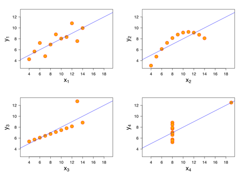
The model generally assumes that the 'errors' are i.i.d. (independant and identically distributed).

This is not necessarily an accurate assumption, as the following counter-examples (known as Anscombe's quartet) show:

Rewriting the RSS in vector form we get:

$$ \frac{1}{2} (y - X\beta)^T (y - X\beta) = \frac{1}{2} \beta^T (X^TX) \beta - \beta^T(X^Ty) $$

Taking the derivative wrt $\beta$ and setting to zero we again get the normal equations:

\begin{split} X^TX \beta &= X^T y \newline \beta &= (X^TX)^{-1} X^T y \end{split}

If the data vectors $x_i$ are linearly independant then the matrix $X^TX$ will be positive definite and therefore invertible. However in general we will use optimization methods such as Newton-Raphson for calculating $\beta$.

Returning to our problem statement $y = Ax$, most real-world phenomena have the effect of low-pass filters in the forward direction. $$ $$ Therefore in solving the inverse-problem, $A^+$ operates as a high-pass filter with the undesirable tendency of amplifying noise: the largest singular values in the reverse mapping were the smallest in the forward mapping. $$ $$ In addition, ordinary least squares implicitly nullifies every element of the reconstructed version of $x$, $\beta$ that is in the kernel of $A$, rather than allowing for a model to be used as a prior for $\beta$.

Tikhonov regularization (aka ridge regression) adds to the linear least squares model a second constraint that $\|\beta\|^2$ cannot greater than a given value: $$ \min_{\beta \in \mathcal{Im}(X),\|\beta\|^2 \leq c } \|y - \beta\|^2 $$ Equivalently, we may solve an unconstrained minimization of the least-squares penalty with $\lambda\|\beta\|^2$ added, where $\lambda$ is a constant (this is the Lagrange multipliers form of the constrained problem):
$$ \min_{\beta} \|y - X\beta\|^2 + \lambda\|\beta\|^2 $$

In a Bayesian context, this is equivalent to placing a zero-mean normally distributed prior distribution on the parameter vector $\beta$: $$ p(\beta) = \mathcal{N}(0,\tau^2) $$ where $\frac{1}{\tau^2}$ controls the strength of the prior.

Our probability model then becomes:

$$ p(y, \beta | x) = p(y | x, \beta) p(\beta) = \mathcal{N}( \beta^T x, \sigma^2) * \mathcal{N}(0,\tau^2) $$

The corresponding MAP estimation problem is equivalent to the Lagrange multipliers form of the constrained optimization problem above:

\begin{split} L(\beta) & = \sum_{i=1}^N \log (p(y_i| x_i, \beta)p(\beta) ) \newline & = -\frac{N}{2} \log(2 \pi \sigma^2) -\frac{1}{2 \sigma^2} \sum_{i=1}^N (y_i - \beta^T x_i)^2 -\frac{1}{2} \log(2 \pi \tau^2) -\frac{1}{2 \tau^2} \sum_{i=2}^n (\beta_i)^2 \newline & \propto \|y - X\beta\|^2 + \lambda \|\beta\|^2 \end{split} where the parameter $\lambda = \frac{\sigma^2}{\tau^2}$.

Note that the second sum generally starts at $i=2$ due to the presence of an unpenalized offset term.

The solution is a regularized version of the normal equations (hence the name Tikhonov regularization): $$ \beta = (X^TX + \lambda I)^{-1} X^T y $$ where $I$ is the $n \times n$ identity matrix. $$ $$ These equations are preferable to solve numerically, especially if $X$ is poorly conditioned or rank-deficient (as is the case when several of the features are highly correllated). Note also the connection with the Tikhonov regularization form of the psuedoinverse.

Using the SVD of $X$, we have that: \begin{split} X\beta &= X(X^TX + \lambda I)^{-1} X^T y \newline &= U\Sigma V^T (V\Sigma^2V^T + \lambda I)^{-1} V\Sigma U^T y \newline &= U \Sigma (\Sigma^2 + \lambda I)^{-1} \Sigma U^T y \newline &= \sum_{i=1}^n \frac{\sigma_i^2}{\sigma_i^2 + \lambda}u_i u_i^T y \end{split} Like linear regression, ridge regression expresses $y$ in terms $U$.

It then shrinks these coordinates by the factors $ \frac{\sigma_i^2}{\sigma_i^2 + \lambda}$, penalizing the basis vectors associated with smaller singular values.